| Table of Contents |
|---|
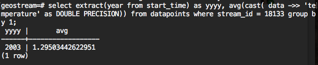
Method 1: Group by extracted time component
This SQL statement is computing average of the bins which created by grouping the extracted time component
Explanation of the SQL:
"where" statement contains the filtering, it should include the stream_id (sensor_id), could include start time, end time, source .....
...
then we just need to convert each SQL result to a json.
Limitation
- Monthly, daily binning will not work. For example, it will group all "December" regardless of year.
- Customized binning, such as water years, can not be used.
Method 2: Group by pre-generated bins with join
This SQL statement pre-generate bins using "generate_series()" and tstzrange type; then it joins with datapoints table and groups by bins
| Code Block | ||
|---|---|---|
| ||
with bin as (
	select tstzrange(s, s+'1 year'::interval) as r
	from generate_series('2002-01-01 00:00:00-05'::timestamp, '2017-12-31 23:59:59-05'::timestamp, '1 year') as s
)
select
	bin.r,
	avg(cast( data->> 'pH' as DOUBLE PRECISION))
from datapoints
right join bin on datapoints.start_time <@ bin.r
where datapoints.stream_id = 1584
group by 1
order by 1; |
Method 3: Group by pre-generated bins with filter for aggregate function
This SQL statement pre-generate bins using "generate_series()" and tstzrange type; then it uses filter with avg function instead of join
| Code Block | ||
|---|---|---|
| ||
with bin as (
	select tstzrange(s, s+'1 year'::interval) as r
	from generate_series('2002-01-01 00:00:00-05'::timestamp, '2017-12-31 23:59:59-05'::timestamp, '1 year') as s
)
select
	bin.r,
	avg(cast( data->> 'pH' as DOUBLE PRECISION)) filter(where datapoints.start_time <@ bin.r)
from datapoints, bin
where datapoints.stream_id = 1584
group by 1
order by 1;
|
Performance
Tested with GLGT production database. Used the stream_id 1584 which has 987,384 datapoints. Used "explain analyze"
| Method 1 | Method 2 | Method 3 | |
|---|---|---|---|
| Planning time | 0.269 ms | 0.259 ms | 0.145 ms |
| Execution time | 3069.059 ms | 6029.105 ms | 12008.801 ms |